Breeden–Litzenberger (BL)

Using the discovery endpoints discussed in the Workflow section, let's investigate some data from the Breeden-Litzenberger set.

# pip install matplotlib numpy
import matplotlib.pyplot as plt
from datetime import datetime, timezone
import numpy as np

# Breeden-Litzenberger.
metric = "bl"
# S&P 500 index.
ticker = "SPXW"
# 2026-01-30 21:00:00 UTC, CBOE closing time.
expiry = "1769806800"
# 2026-01-27 11:45:56 UTC
measurement_time = "1769514356"

# Get the data from Reflex Research.
data = get_measurement(
    metric,
    ticker,
    expiry,
    measurement_time,
)

# Visual check of data.
print(data)

# Quick check of some statistics.
x = np.asarray(data["payload"]["data"]["underlying"], dtype=float)
pdf = np.asarray(data["payload"]["data"]["pdf"], dtype=float)

# This should be very close to 1, as it represents a probability
# distribution.
area = np.trapz(pdf, x)

# Underlying price where the PDF is a maximum.
mode_x = x[np.argmax(pdf)]

# Standard deviation.
mean_x = np.trapz(x * pdf, x)
var_x = np.trapz((x - mean_x) ** 2 * pdf, x)
std_x = np.sqrt(var_x)

# Skewness.
skew_x = np.trapz(((x - mean_x) / std_x) ** 3 * pdf, x)

print("Area:", area)
print("Mode:", round(mode_x, 2))
print("Mean:", round(mean_x, 2))
print("STD:", round(std_x, 2))
print("Skew:", round(skew_x, 2))

# Get measurement time for display.
meas_dt = datetime.fromtimestamp(
    data["measurement_time"], tz=timezone.utc
).strftime("%Y-%m-%d %H:%M:%S")

# Get expiry time for display.
exp_dt = datetime.fromtimestamp(
    data["expiry"], tz=timezone.utc
).strftime("%Y-%m-%d %H:%M:%S")

plt.figure(figsize=(10, 6))
plt.plot(x, pdf, lw=2)
plt.xlabel("Underlying price")
plt.ylabel("Probability density")
plt.title(
    "Breeden-Litzenberger Probability Density\n"
    f"{data['ticker']} | Measured {meas_dt} UTC | Expiry {exp_dt} UTC"
)
plt.grid(alpha=0.3)
plt.tight_layout()
plt.show()

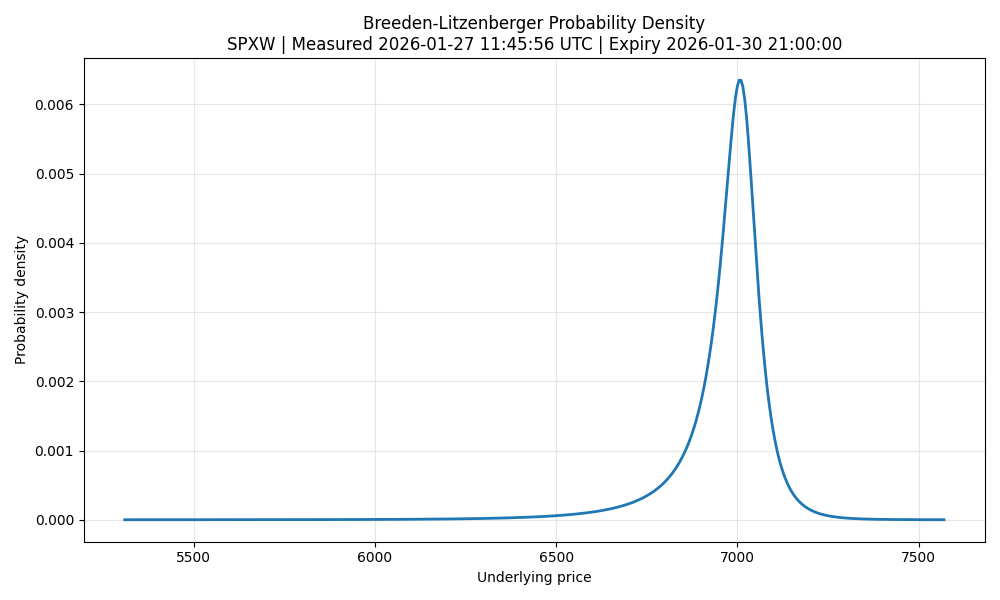
For this example, the following statistics were obtained:

Area: 0.9999366831449135
Mode: 7005.0
Mean: 6969.2
STD: 124.01
Skew: -2.57

This data gives some useful insights into what the market is pricing in, for the expected value of the S&P 500 at the end of the trading day of 2026-01-30. The negative skew indicates a fat tail distribution where downside risk is anticipated.

A plot of the data is shown below.